Institute of Bioinformatics Münster
MetaG
About
Usage
Tutorial
Preprint
Run
View results
View testcases
Download
GitHub
Contact
News 
2025-01-22
Updates for all databases, except RDP2024-01-10
Updates and new standards for non-viral databases2023-09-18
Updated filter database to T2T-CHM13v22023-06-07
Updated RefSeq and BV-BRC (formerly: PATRIC)2023-06-02
Updated ICTV2023-03-17
Updated ICTV2022-11-24
Updated ICTV2022-09-16
Updated ICTV2022-06-30
Query can be a nested archive2022-05-14
Updated ICTV2022-04-27
MTX now uses NCBI taxonomyTutorial
Welcome to MetaG
MetaG assigns a taxonomy to reads from marker genes data, e.g. of the 16S rRNA gene, and to
reads from WGS (viruses). MetaG is applicable to both short and long reads: It has been tested on
Nanopore and Illumina MiSeq data.
Concepts and parameters
Input data
The software currently supports fasta or fastq data which means your data should like this (fasta):
>seq1
ATGCATG
>seq2
ATGCCTGG
or like this for fastq:
@seq1
ATGCATG
+
,,..;;!
@seq2
ATGCCTGG
+
..;;!!$%
The file format will be detected automatically. Please make sure that your sequences don't contain
special characters like "-" or "?". Please note that the query file must be one file. However, you
may compress multiple fasta/fastq files into one .tar, .gz, .zip or .bz2 file. Currently, the file size limit
for a single fasta/fastq file or for the whole archive is 6 GB. It is also possible to submit nested archives:
For example, you can compress multiple *.fastq.gz files into a single ZIP archive. Please make sure that all files
in the archive(s) have unique names.
Principle of MetaG
Choose Run from the menu to start your analysis. In the section Standard workflow, you will learn how to set the
standard parameters for short and long-read technologies. But first, you need to get a glimpse of what MetaG is doing
so you can understand the parameters and their influence on your analysis.
If you decide to filter your reads (see Filter reads), only reads that pass the filter will be assigned with a
taxonomy. Otherwise, this is attempted for all reads. The taxonomy calling consists of two parts. First, your sequenced
reads are compared (aligned) to a reference database by using LAST. The database contains sequences with a known
taxonomy. This comparison would just leave you with a bunch of comparisons between your individual read and database
entries. The amount and significance depends on the parameters you chose (alignment parameters).
The second part (taxon calling) makes use of these comparisons: By setting an e-value and alignment score cutoff
you take a subset of the comparisons for each read (or discard all, if your settings were too strict :) ).
A small e-value and a high alignment score are strict. This means you can be more confident in your
results. You enter the exponent of the e-value to the respective field, which means that a low negative number will be
strict. For example, you choose -3. Internally, this is recognized as e^-3. Choosing -5 (translated to e^-5) is more
strict, because e^-5 < e^-3. For the alignment score you enter a decimal value, e.g. 0.5. The alignment score depends on
the best alignment for a single read (maximum alignment score). All alignments with an alignment score less than max score
* score cutoff will be discarded. Generally, an alignment score cutoff of 1.0 is most strict, while choosing 0.0 will be
pretty relaxed.
In a real-world scenario your alignments for one read will most likely not give you a single taxonomy. This may
be due to sequencing or alignment errors. Maybe you also used alignment parameters which were not optimal. Note, that
short and long-read sequencing technologies need different parameters for alignment and taxonomy calling. You can see
this trend by comparing our standard parameters for Illumina and Nanopore data, respectively (see Standard workflow).
However, the result should be a common (consensus) taxonomy for each of your sequencing reads. To achieve that,
the algorithm compares the database entries in the alignments for each of your reads. The consensus taxonomy is then
inferred by the majority of database entries. Setting the confidence cutoff, allows you to influence how strict you
want the consensus decision to be. A strict cutoff of 1.0 may only give you results at broader taxonomic levels, e.g.
the family level. A loose cutoff of 0.0 may give you a higher resolution at lower ranks, but with less confidence:
Fewer of the matching database entries support that call.
The confidence in an observed taxon will be the average of the individual read's confidences. The method for
average confidence calculation will tell the program how to calculate the average. This parameter is just
for the display and will not influence the calling process itself.
You will also get interactive visualizations made by a customized version of Krona and lots of data to download. Details will be
explained in Understanding the output.
Standard workflow
Upload your sequenced reads in fasta/fastq format by clicking the Query File field. Choose one of the databases
MTX_SSU_LSU or RDP_16S_28S, RefSeq_Arch_Bac_Fung or ICTV_virus (further details on the databases are below) using the Database
menu (Figure 1). After you chose a database, you can choose a standard profile for the analysis ( Database
Profile) (Figure 1). We offer standards for Illumina and Nanopore sequencing (short and long-read technologies,
respectively). You can load your own parameters from a file by choosing "Load from local file" (see also Usage, section
2.9.3). If you want to use your own parameters, use LAST-TRAIN to figure out optimal parameters for the substitution
matrix and alignment. Additionally, you could set LAST-SPLIT (-m) to filter ambiguous alignments.If you want to
read about parameter choice in detail, visit the LAST website. If you don't want to load a
file, you can type your parameters by clicking on Advanced Parameters.
Optionally, you may want to enter your email address to get a notification when your job is finished. IMPORTANT:
If you provide no email address, you have to remember your request ID or stay on the website. Providing a
recognizable title for your job may also be a good idea (Figure 1).
Submit your job by clicking
Run
.
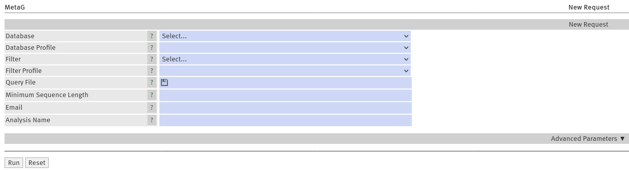
Figure 1: Webinterface of MetaG
Filter reads
If your sample contains a high amount of DNA that is not interesting for your analysis
(e.g. host DNA in a viral analysis), you may want to filter these reads out. If you remove the "contamination", your
output will be more focused on your taxa of interest. This results in nicer graphs and reduced false positive
classifications. To filter your reads, simply select a filter database ("Filter", Figure 1) and a parameter set
("Filter Profile", Figure 1) according to your sequencing technology. Generally, the sequencing technology selected here,
should match the technology selected under "Database Profile". Currently, you will not be able to use custom
filter settings. Choose all other parameter, like described in the previous section. Internally, your input reads will
first be aligned to the filter database. Any unaligned reads (reads passing the filter) will be assigned with a
taxonomy, if possible.
Databases
The algorithm uses RDP containing 16S rRNA, 28S rRNA
genes and ITS from bacteria, fungi and archaea. The MTX database (obtained from Metaxa 2.2) contains LSU and SSU genes. MTX is
smaller than RDP, thus the analysis is faster. Please choose MTX first, if you plan to submit whole genome
reads (experimental). Besides, MTX contains many sequences from organelles, e.g. from chloroplast or mitochondrion.
Choose MTX if you expect eukaryotes other than fungi. Both databases were heavily customized to provide a
better resolution on the species level!
RefSeq is our recent addition to MetaG. Like MTX, it is a rather small and highly curated database. A smaller
database typically means a faster calculation time (at the expense of some resolution). This makes it especially useful
when dealing with large samples. Our RefSeq version was build from the Targeted Loci project. It contains bacterial (16S, 23S, 5S
rRNA), archaeal (16S, 23S, 5S rRNA) and fungal sequences (18S, 28S rRNA, ITS).
Interested in viruses? With ICTV, we provide a great
database for whole-genome analysis of viruses.
Filter databases
If you choose the filter workflow, reads are filtered using human genome T2T-CHM13v2 which we obtained from RefSeq.
Understanding the output
Once your request is finished, you will receive an email. If you did not provide your email
address, you have to enter your request ID. Go to "View results", enter your ID in the respective field and
click "Goto". If you have not yet generated your own results, you can view a testcase. Choose "View testcases" from
the menu and select a testcase of your choice. In the following you will get to know all output data.
Info
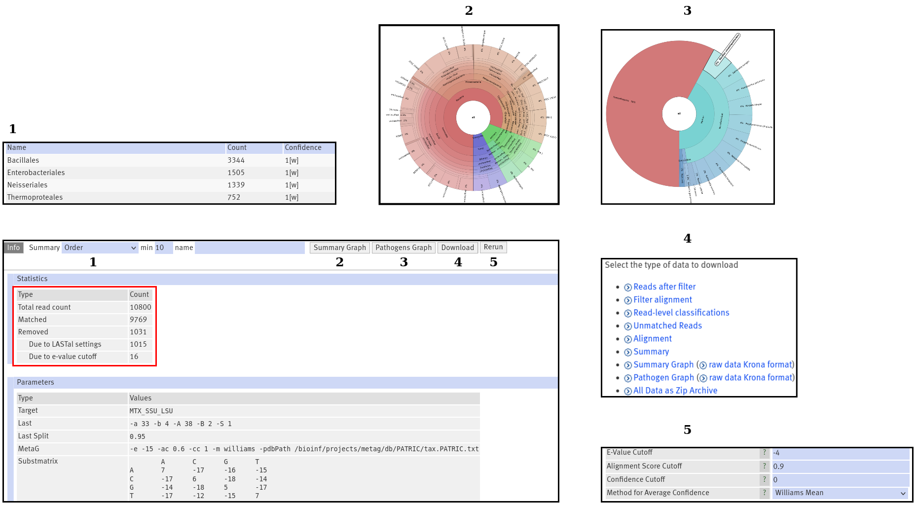
Figure 2:The "Info" output. Pressing the numbered buttons, displays the output in the numbered boxes.
If you open your results, you will start in the Info section which will provide you with general information, like
runtime and your chosen parameters. Also, you will find an overview
over the total read number in your fasta/fastq file and how many reads were assigned with a taxon. Another interesting number
is the number of removed reads. You will see how many reads were removed, because the alignment was to weak. Additionally,
your e-value cutoff might have removed some reads (see also Figure 2, red box). Remember, the alignment score cutoff depends on the very best match
for each read and will not lead to any read loss.
These values are interesting because you can use them to tune your analysis. For example, if you
have high quality reads from the marker genes present in the respective database (targeted sequencing), the number of removed
reads should be small. However, if you have whole genome sequencing data, you may want to increase that number. This follows the
idea that the marker gene will be represented by only a fraction of your reads. Thus, to avoid spurious assignments, not all reads
should match the database.
Summary
The summary table opens by clicking on the dropdown menu (Figure 2: 1). It contains the abundance (i.e. read count) and confidence
for each identified taxon. The method for average confidence calculation is abbreviated behind the confidence value. You can select the rank that you
want to display from the menu. Directly next to it, a minimum abundance for taxa at the current rank can be entered. This may help to filter
spurious taxa and to make the results more clear; especially on the strain level. By default, the minimum abundance is 10. With the name field,
you can search the table. The search function uses a style which is similar to the regular expression syntax. This is really not as complicated
as it may sound. Imagine you want to search the table for "bacillus" at the genus. Surprisingly, you get hits to Bacillus, Thiobacillus, Paenibacillus,...
If you type "^bacillus", you will get only matches starting with bacillus. This was probably what you expected from results of your first hypothetical
search. Likewise, "bacillus$" provides matches ending with bacillus. The search algorithm is not case-sensitive. To search for multiple terms,
separate them by commas. The UNMATCHED taxon sums up reads that could not be assigned with a taxonomy at the given rank due to the confidence
cutoff or other taxonomic ambiguities. Please don't confuse this with unclassified. Taxa are unclassified, if the database does not assign any
name at that rank: A bacterium which belongs to an unknown genus is unclassified at genus level.
Summary Graph
This is an interactive visualization of the summary table (see also Figure 2: 2). You can double click on any label and
the graph will reshape. The graph displays the broadest ranks (e.g. domain) in the inner circles. The further you go to the rim of the chart, the
more specific the rank. Double clicking on a rank allows you to set this as the inner circle. Thus, the outer fields connected to this
taxon will expand. All other fields will be hidden. To go back, click on the respective pie chart on the right or choose a taxon from
the short list in the middle. The left panel contains several options to customize the view: The Max depth influences the amount of
ranks that are displayed. By default, you can see all ten ranks. If you set it to nine, the most specific rank (here: strain) will no longer
be displayed. You can also collapse the view: If one domain only has one strain, only the strain field is shown and the fields for the
ranks between domain and strain are hidden. Both will improve the performance, especially if you have many taxa (from unique lineages).
Try it yourself!
You can also search the graph via the search bar. However, taxa that are currently hidden (collapsed or removed by max depth)
cannot be found. This is why we show all ranks by default and don't collapse the chart.
Pathogens Graph
This works exactly like the summary graph. It displays the results of the search for pathogens. If you used the MTX, RDP or
the RefSeq database, pathogenic bacteria and archaea are looked up in
BV-BRC (formerly: PATRIC) (see also Figure 2: 3). The inner circle represents the host. Currently, only human is
supported. The middle ring is showing the antibiotic resistance. The species names are given on the outer ring. Nonpathogenic represents
non-pathogenic organisms or those that could not be found in the database.
The percentages in the diagram are probabilities. To assign an absolute value, strains would have to be queried in BV-BRC.
However, due to nomenclature clashes and detection issues, species names are queried. Thus the probability of observing a species with a
certain host and resistance (phenotype) is given. The value integrates the abundance of the taxon in your sample and the number of reports
for a certain phenotype in the database. Taxa with non-informative species names, e.g. uncultured bacterium, cannot be queried and are
assigned to Nonpathogenic.
When using ICTV, information about pathogens is retrieved from ICTV itself. The pathogens graph will only display the host
probabilities for the viral species (see also above).
Download
For in-depth analysis or sharing with your colleagues, you can obtain all output data (see also Figure 2: 4). These are the
two graphs, the input files used in Krona to create the charts and the summary. The summary file contains the table from the section "Summary",
as well as the read counts from the "Info" section. The taxonomic assignment of the individual reads is in the "Read-level classifications" file.
We also provide the unmatched and filtered (if you used the filter workflow) reads, as well as the alignment files. One alignment file is
related to the filter workflow, the other to the taxonomic assignment. You can also download all results at once as a ZIP archive.
Rerun
With this button, you may perform the taxon calling again (see also Figure 2: 5). This is performed on your old alignment.
Since the generation of the alignment is the most time consuming step, this will be fast. However,
you may only adjust "E-Value Cutoff", "Alignment Score Cutoff", "Confidence Cutoff" and the "Method for Average Confidence". If you
want to adjust any of the alignment parameters including, matrix and LAST-SPLIT -m, or the database, you need to submit a new job. You also
need to submit a new job to change the filter settings.
WARNING: Rerunning will delete your previous results. If you want to compare the results
of both runs, you must first download your current results.
Tips and tricks
My analysis is slow
Consider reducing the amount of input data, i.e. less sequencing reads.
Have you already tried to use the MTX or RefSeq database? Both are smaller than RDP and thus also faster.
I get a lot of unexpected taxa
This may very well be due to "contamination" of your sample with host DNA. We found that analyzing human
samples with ICTV can lead to unexpected calls of Zika virus. To get rid off host DNA, please follow the steps outlined in
the section "Filter reads" of the tutorial.
Number of matching reads influences the quality
The read counts on the info page (see also Understanding the output), tell you
how many reads were assigned with a taxonomy. For the assignment of non-viral reads, reads are looked up
in a database of selected genes (see also Concepts and parameters). If you provide data from whole-genome
shotgun sequencing, most of the reads are not expected to be from these genes. Thus, spurious reads should be removed
from the analysis. You may tune the parameters of LAST or the taxon calling (i.e. "E-Value Cutoff",
Alignment Score Cutoff", "Confidence Cutoff") to increase the number of removed reads. In the case of targeted
sequencing of a marker gene that is present in the respective database, you may try to avoid loosing too many reads.
However, this also depends on the quality of your sequencing data.
Quickly rerunning the pipeline
By clicking Rerun in the results window (see also Understanding the output) you may perform the taxon calling again.
This is performed on your old alignment. Since the generation of the alignment is the most time consuming step,
this will be fast. The downside is, that you may only adjust "E-Value Cutoff", Alignment Score Cutoff", "Confidence Cutoff"
and the method for average confidence calculation. If you want to adjust any of the alignment parameters including, matrix
and LAST-SPLIT -m, or the database, you need to submit a new job. You will also need to submit a new job, if you want to
change the the read filtering
WARNING: Rerunning will delete your previous results. If you want to compare the results
of both runs, you should first download your current results.
What can I do, if I got an "error during alignment"?
Please check that your input sequences don't contain special characters like "?" and "-".
Something is unclear?
Write to the developers using the "Contact" button. We can help you more easily, if you provide a detailed
description of your problem. We are also happy about suggestions to make the tutorial more clear.
2024-11-04 16:23